A Probability Is a Price
The ledger says Minnesota beats Green Bay with probability .5970. That is a sentence about football, but it is also, unavoidably, a sentence about money: any probability implies a spread and a price, and once you write those down you can check them against what the market was charging. This page does the conversion for all sixteen 2026 openers, using a points-to-probability relation fitted on this file rather than assumed, and then does the thing that makes the exercise honest — it runs the same procedure on sixteen seasons of stored closing prices to see whether the model's "edges" have ever been worth anything.
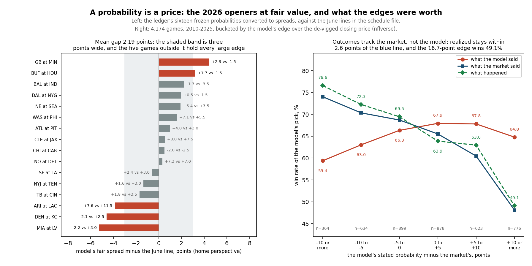
The short answers. A 60% pick is worth 3.03 points of spread and a moneyline of about −148. Measured against the June lines the schedule file carries, the model's sixteen fair spreads sit a mean of 2.19 points from the market's, with five games more than three points apart, and eight of the sixteen picks would carry positive expected value at the stored prices — two of them enormously. And then the audit: backing this model's pick in all 4,174 regular-season games since 2010 that carry both moneylines loses 54.7 units, or 1.31% a bet, which is almost exactly the cost of the margin and nothing else. In the bucket where the model claims the biggest edge, an average of 16.7 percentage points over the de-vigged price, its pick has won 49.1% of the time.
So the fair prices below are real arithmetic and the expected values are real arithmetic, and the sixteen-season record says the inputs are not good enough for either to mean what it looks like it means. That is worth publishing in full, before kickoff, rather than after.
Turning a Probability into Points
There are two defensible ways to convert, and this site already published the ingredients for both. The spread-accuracy page measured the scatter of actual margin around the closing line: mean error +0.094 points across 7,276 games, mean absolute error 10.27, standard deviation 13.20. Treat that scatter as normal and a probability p for the home side implies a margin of 13.20 × Φ−1(p). The alternative is to skip the margin and fit the win directly: a logistic regression of the home team's win on the spread, over the 7,261 decided games that carry a line, which comes out as
p(home wins) = 1 / (1 + exp(-(-0.0265 + 0.14262 × spread))) [SE on the slope: 0.0048]The slope is the useful number: each point of spread multiplies the home side's odds by 1.153, and near a coin flip that is 3.6 points of probability per point. The intercept is −0.027 with a standard error of 0.027, meaning the market's line is unbiased about who wins as well as by how much. Inverting the fit gives a ladder from probability to points:
| Model probability | Fair spread, fitted | Fair spread, normal (13.20) | Fair moneyline |
|---|---|---|---|
| 55% | 1.59 | 1.66 | −122 |
| 60% | 3.03 | 3.35 | −150 |
| 65% | 4.53 | 5.09 | −186 |
| 70% | 6.13 | 6.92 | −233 |
| 75% | 7.89 | 8.91 | −300 |
Fitted column from the logistic above; normal column from the published 13.20-point scatter. Fair moneyline is the zero-margin price of the probability itself: −100 × p / (1 − p).
The two columns agree near a coin flip and diverge past a field goal, by a full point at .75. The file arbitrates. Three-point favorites have won 58.1% of 1,152 games, against 59.9% from the fit and 59.0% from the normal — both fine. Seven-point favorites have won 76.0% of 488, against 72.5% fitted and 70.2% normal; that is three standard errors above the normal curve. Real football margins have fatter shoulders than a normal distribution because they pile up on the key numbers — 15.1% of all games land on exactly 3 and 9.0% on exactly 7, both reproduced here from the same file — so this page uses the fitted column throughout and flags the choice as a choice.
The Exhibit
The Sixteen, Priced
| Game | Model pick | Its probability | Fair spread | June line | Fair price | File's price | EV per unit | Quarter Kelly |
|---|---|---|---|---|---|---|---|---|
| MIA at LV | MIA | 58.6% | −2.2 | +3.0 | −141 | +145 | +43.5% | 7.5% |
| DEN at KC | DEN | 58.1% | −2.1 | +2.5 | −138 | +130 | +33.5% | 6.4% |
| GB at MIN | MIN | 59.7% | +2.9 | −1.5 | −148 | +105 | +22.4% | 5.3% |
| DAL at NYG | NYG | 51.0% | +0.5 | −1.5 | −104 | +110 | +7.0% | 1.6% |
| BUF at HOU | HOU | 55.4% | +1.7 | −1.5 | −124 | −108 | +6.7% | 1.8% |
| WAS at PHI | PHI | 72.8% | +7.1 | +5.5 | −268 | −230 | +4.5% | 2.6% |
| NE at SEA | SEA | 67.9% | +5.4 | +3.5 | −211 | −205 | +1.0% | 0.5% |
| CHI at CAR | CHI | 57.8% | −2.0 | −2.5 | −137 | −135 | +0.6% | 0.2% |
| ATL at PIT | PIT | 63.2% | +4.0 | +3.0 | −172 | −175 | −0.7% | — |
| CLE at JAX | JAX | 75.3% | +8.0 | +7.5 | −306 | −340 | −2.5% | — |
| NO at DET | DET | 73.4% | +7.3 | +7.0 | −276 | −325 | −4.0% | — |
| SF at LA (Melbourne) | LA | 57.9% | +2.4 | +3.0 | −137 | −175 | −9.0% | — |
| NYJ at TEN | TEN | 55.2% | +1.6 | +3.0 | −123 | −170 | −12.4% | — |
| ARI at LAC | LAC | 74.3% | +7.6 | +11.5 | −289 | −625 | −13.8% | — |
| TB at CIN | CIN | 55.7% | +1.8 | +3.5 | −126 | −192 | −15.2% | — |
| BAL at IND | BAL | 55.2% | −1.3 | −3.5 | −123 | −192 | −16.1% | — |
Spreads and the June line are from the home team's perspective (positive = home favored). Fair price is the model's probability expressed as an American moneyline with no margin; the file's price is what the bundled schedule row stores for that side. EV is per unit staked at that price, using the model's probability. Kelly is quartered, and shown only where the expected value is positive.
The board's five widest disagreements are the whole story: Miami at Las Vegas (5.2 points), Denver at Kansas City (4.6), Green Bay at Minnesota (4.4), Arizona at the Chargers (3.9) and Buffalo at Houston (3.2). Four of the five are games the predictions page already flagged as quarrels with the market; what the price conversion adds is the size of the claim. On the moneyline the model is asserting a 19.5-point probability edge on Miami and 16.35 on Denver, the second of which is the number the Chiefs page published from the same two sources.
Two housekeeping notes before anyone takes the EV column seriously. The sixteen June moneyline pairs carry an average hold of 4.31% — the figure the road-favorites page reports, and unusually fat; the 4,174 historical pairs in the same file average 2.90%. And the model's own numbers, taken at face value, say that backing all sixteen picks returns +2.8% a bet, which would be a spectacular business if the numbers were true.
Sixteen Seasons of Exactly This Procedure
They are not true. The engine has been walked forward over the full game log since 1999 and graded since 2010; 4,174 of those graded regular-season games carry both moneylines, which means the identical calculation can be run on all of them with the model blind to the price. Flat one unit on the model's pick, every game:
- −54.7 units over 4,174 bets, or −1.31% a bet with a standard error of 1.22% (z = −1.07). It is not a catastrophe; it is the margin. Half the average hold is 1.45%, and a bettor with no information at all loses exactly that.
- Six of sixteen seasons finished positive, the best +26.2 units in 2015 and the worst −25.8 in 2021. Sixteen seasons of variance around a small negative number looks like this.
- Backing the market's own favorite instead loses 2.64% a bet — twice as much, because favorites carry more juice per unit of edge. The model is not worse than a naive rule; it is simply not better than zero.
- Against the spread, converting each model probability to a fair margin and taking the side of the number, the record is 2,042–2,027–106, a 50.18% win rate where standard −110 juice needs 52.38%. That is a 2.2-point shortfall and −170.6 units. It also matches what this site found about cover rates generally: knowing who wins is not the same as beating the number.
The interesting part is not the total. It is what happens when you sort by how big the model thought its edge was.
Where the Edges Went
| Model's edge over the de-vigged price | Games | Model said | Market said | Actually won | Units per bet |
|---|---|---|---|---|---|
| −10 points or worse | 364 | 59.4% | 74.0% | 76.6% | +0.5% |
| −10 to −5 | 634 | 63.0% | 70.3% | 72.3% | +0.1% |
| −5 to 0 | 899 | 66.3% | 68.7% | 69.5% | −1.6% |
| 0 to +5 | 878 | 67.9% | 65.5% | 63.9% | −5.7% |
| +5 to +10 | 623 | 67.8% | 60.5% | 63.0% | +1.8% |
| +10 points or better | 776 | 64.8% | 48.1% | 49.1% | −0.4% |
Regular-season games 2010–2025 with both moneylines stored, bucketed by the model's stated probability for its own pick minus the market's proportionally de-vigged probability for that same side. "Actually won" excludes the 13 ties.
Read the last three columns across. The realized rate never departs from the market's stated probability by more than 2.6 points in any bucket, and it departs from the model's by up to 17.2. In the bottom row the model believes it has found 16.7 points of value, the market prices those picks at 48.1%, and they win 49.1% — the market, to within one point, on 776 games. In the top row the model is the pessimist, calling a 59.4% side that the market makes 74.0%, and the side wins 76.6%. Whenever the two disagree, the outcomes side with the price.
The formal version of that observation is a forecast-encompassing regression in the manner of Fair and Shiller: put both stated probabilities, on the log-odds scale, into one logistic model of the outcome. The market's coefficient comes out at +1.040 (SE 0.079), indistinguishable from the perfectly calibrated 1.0. The model's comes out at +0.033 (SE 0.078), indistinguishable from zero. Given the price, this model adds nothing. On its own it is not useless — its solo slope is 0.898, and it calls 64.6% of games against the market's 66.6% — but its information is a subset of what the line already contains, and its solo slope being two standard errors under 1.0 says it is also overconfident. The Brier scores agree: .2205 for the model, .2104 for the market, with log losses of .6326 and .6099.
Worked Example: The Board's Biggest Number
Miami at Las Vegas, end to end. The ledger states the home side, so the number to convert is Las Vegas at .4143. Its log-odds are −0.3463, and (−0.3463 + 0.0265) / 0.14262 = −2.24: a fair line of Miami by 2.2, written from the home team's side as the table does. The file has Las Vegas favored by 3, so the two disagree by 5.2 points, the widest gap on the board. Miami's fair moneyline is −100 × .5857 / .4143 = −141; the file offers +145, decimal 2.45.
Expected value per unit is then .5857 × 1.45 − .4143 = +0.435, and the Kelly fraction is that divided by the 1.45 you win, or 30.0% of a bankroll on one September football game. Quarter Kelly, the usual concession to the fact that nobody's probabilities are that good, still asks for 7.5%. Add up quarter Kelly across the eight positive sides and the board wants 25.9% of a bankroll staked in a single weekend.
That number is the argument against itself. A 43.5% edge does not exist in a market with 4.31% of margin in it; what exists is a 19.5-point disagreement between a rating system that has not seen a roster since February and a price that has. The bucket table says disagreements of that size have won 49.1% of the time. The correct reading of the Miami row is not "the model found value" but "the model and the market are 19.5 points apart, and history says that gap measures the model's blind spot rather than the market's."
What This Page Cannot Tell You
- These are not closing lines, and they are not today's. Every 2026 number here is the June snapshot bundled in the schedule file. Lines move for months; by Wednesday night some of these will be several points different, and the fat 4.31% hold is itself a sign of an early, thin market. Nothing in the 2026 table should be read as a live quote.
- Sixteen games settle nothing. The standard error on a 16-bet sample is enormous; the model could go 12-4 this week and it would not move the sixteen-season verdict by a measurable amount. The historical audit is the evidence on this page. The 2026 table is an illustration of the arithmetic.
- The historical prices are as stored, not as available. The file's moneylines are one recorded number per game; they carry no timestamp, no book, no line-shopping and no limits. A real bettor faces worse prices than the best number and better than the worst, and this test can model none of that.
- The conversion is a choice. The fitted logistic and the normal model disagree by a full point at .75, and both ignore the lumpiness at 3 and 7 that gives half-point moves their real value. Every fair spread above would shift by a few tenths under a different, equally defensible fit.
- Kelly assumes the probability is right. The formula is Kelly's, from 1956, and it is optimal only for a true probability. Fed an overconfident one — and the solo slope of 0.898 says these are overconfident — it recommends stakes that are not merely aggressive but negative-expectation.
- This is analysis, not advice. Nothing here is a recommendation to place a bet, and the page's own conclusion is that the model has no demonstrated edge over the market price. The site publishes probabilities and grades them; it does not tip.
Reproduce It
Two published files: games.csv from nflverse nfldata, bundled at /data/games.csv with spreads and moneylines as recorded, and the frozen ledger at /data/predictions.json. The harness is explainer_src/make_fair_price_chart.py. The conversion itself is four lines:
import numpy as np, pandas as pd

d = pd.read_csv("data/games.csv").dropna(subset=["home_score", "spread_line"])
d = d[d.home_score != d.away_score]
X = np.column_stack([np.ones(len(d)), d.spread_line])
y = (d.home_score > d.away_score).astype(float).values
b = np.zeros(2)
for _ in range(40):                                  # Newton-Raphson
    p = 1 / (1 + np.exp(-X @ b))
    b += np.linalg.solve(X.T @ (X * (p * (1 - p))[:, None]), X.T @ (y - p))
print(b)                                             # [-0.02647  0.14262]

fair_spread = lambda q: (np.log(q / (1 - q)) - b[0]) / b[1]
fair_price  = lambda q: -100 * q / (1 - q) if q >= .5 else 100 * (1 - q) / q
print(fair_spread(0.5970), fair_price(0.5970))       # 2.94 points, -148
The script asserts every figure on this page — the logistic fit and its standard errors, both ladders, the empirical rates at 3 and 7 points and the key-number frequencies, the sixteen fair spreads and prices with their expected values and Kelly fractions, the average holds, the 4,174-game flat-betting result with its standard error and per-season range, the against-the-spread record, all six edge buckets, and the encompassing regression: 103 assertions, all green as of September 7, 2026.
Sources: the nflverse public game log bundled at /data/games.csv; probabilities from explainer_src/nfl_elo.py, the module that writes the live ledger, imported rather than reimplemented. The encompassing test follows Ray C. Fair and Robert J. Shiller, "Comparing Information in Forecasts from Econometric Models" (American Economic Review, 1990); the staking formula is from J. L. Kelly Jr., "A New Interpretation of Information Rate" (Bell System Technical Journal, 1956).
Further reading
- The Offseason Haircut — today's companion: where the sixteen probabilities on this page came from, and how much of them is a constant
- How Accurate Is the Point Spread? — the 13.20-point scatter this page's normal conversion is built on
- Key Numbers — why the margin distribution is lumpy, and why that breaks any smooth conversion at 3 and 7
- Do Big Favorites Cover? — the cover-rate version of this page's against-the-spread result
- Road Favorites — the de-vigged market board for these same sixteen games, in probabilities rather than prices
- The 2026 Week 1 Predictions — the sixteen decomposed into ratings, and the five quarrels with the market this page prices
- Win Probability, Explained — what a probability is before anyone attaches a price to it
- The Model, Fully Stated and the ledger — the engine being audited here, and its public grade
Go deeper
Want the code behind these metrics? Work through the 43-chapter NFL analytics tutorial.
Browse tutorials Free tools