The Question: Is Winning Close Games a Skill?
Every winter the same sentence gets written about somebody: "they just know how to win the close ones." It's a checkable claim, and this page checks it. From the bundled nflverse game log — 6,967 played regular-season games, 1999–2025 — I split every game by final margin: one-score (decided by 8 or fewer, the same cutoff as our one-score frequency page) and blowout (17 or more). That's 3,543 one-score games (50.9%) and 1,869 blowouts (26.8%): the average team plays 8.2 one-score games a season, half its schedule. The test is the simplest one that could work: line up the same franchise in back-to-back seasons — 829 season-pairs — and ask which stats carry over. A skill should correlate with itself a year later. A coin shouldn't.
The Exhibit: The Same Franchise, One Year Apart
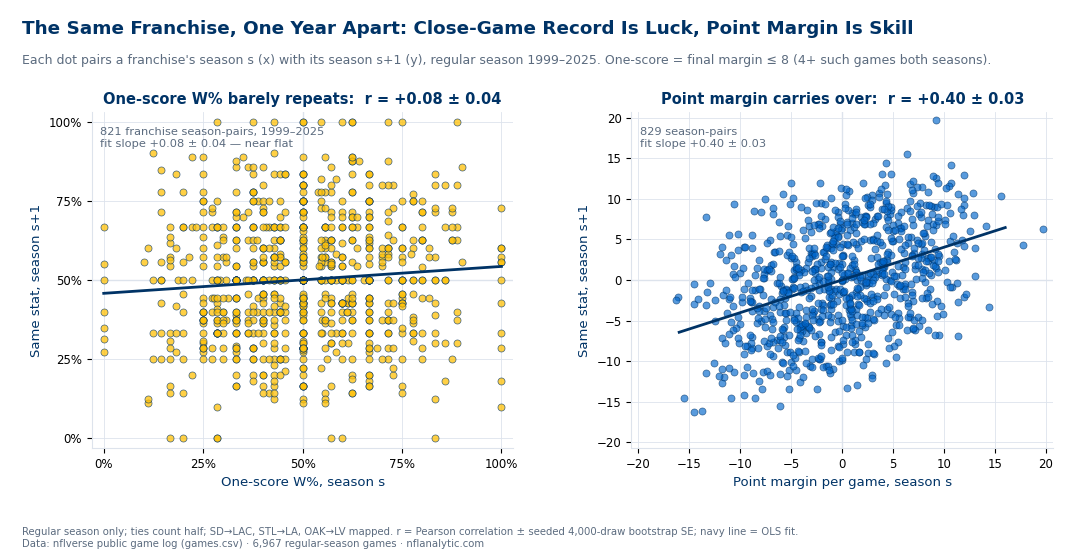
Both panels plot every franchise against itself, season s on the x-axis, season s+1 on the y. If a stat is skill, the cloud tilts. One-score record (left, 4+ close games in both seasons) doesn't tilt; point margin (right) does.
And here is what happened, one year later, to the best close-game seasons since 1999 (8+ one-score games):
| Season | Team | One-score | Overall | One-score, next year |
|---|---|---|---|---|
| 2024 | Kansas City | 11-0 | 15-2 | 1-9 |
| 2022 | Minnesota | 11-0 | 13-4 | 6-8 |
| 2009 | Indianapolis | 8-0 | 14-2 | 5-4 |
| 2012 | Indianapolis | 9-1 | 11-5 | 6-1 |
| 2024 | Minnesota | 9-1 | 14-3 | 5-4 |
| 2017 | Carolina | 8-1 | 11-5 | 3-7 |
| 2001 | Chicago | 8-1 | 13-3 | 4-6 |
| 2008 | Indianapolis | 8-1 | 12-4 | 8-0 |
The ten best one-score seasons in the file averaged a .549 close-game record the following year. Only Peyton Manning's 2008–09 Colts sustained it — and one repeat in a list built by selecting extremes is what chance predicts, the same survivorship arithmetic the streaks page runs on winning runs.
The Honest Read: Four Correlations and a Coin
The persistence ladder. Year-over-year, across the same 829 franchise pairs: point margin per game r = +0.40 (±0.03), record in non-close games +0.37 (±0.03), blowout record +0.35 (±0.04), overall record +0.33 (±0.03)… and one-score record +0.08 (±0.04). Every stat that measures how hard you hit repeats; the one that measures which way the tight ones bounced doesn't. The ordering itself is the finding: overall record persists worse than its non-close component because half of every record is one-score noise.
The variance test agrees. If close games were literal coin flips, the spread of close-game records across 856 team-seasons would be an SD of .180 (given each team's game count). Observed: .194 — just 8% wider than pure chance. Blowout records, by contrast, run 41% wider than their coin baseline. Within a single season teams do differ in close games about as much as coins differ from coins.
And close-game record predicts nothing beyond margin. This is the load-bearing test. One-score record does correlate +0.15 with next season's overall record — but only because good teams are modestly better in close ones in the moment (same-season r with margin: +0.47). Put both in one regression — next-season W% on this season's margin per game plus this season's close-game W% — and margin carries a t-statistic of +10.0 while the close-game coefficient is −0.02 (±0.04, t = −0.7): zero, leaning negative. Once you know how a team outscored its schedule, its close-game heroics tell you nothing about next year. This is the mechanism behind Pythagorean regression, measured directly.
The extremes regress on schedule. The 140 team-seasons at .700+ in close games (average .798) came back at .515; the 138 at .300 or worse (average .220) came back at .462. Both landed on the coin, and the heroes' overall records fell from .721 to .549 — nearly three wins of regression. Blowout dominance regressed too (.886 to .650) but stayed far above water: skill dilutes; luck resets. The +0.08 holds at every minimum-game threshold (1+, 6+, 8+ close games: +0.08, +0.05, +0.07) and in both halves of the window (1999–2011: +0.07 ± 0.05; 2012–2024: +0.10 ± 0.05).
Worked Examples, Straight from the File
- The cruelest flip in the file. Kansas City won every one-score game in 2024 — eleven of them — and was crowned inevitable at 15-2. In 2025 the Chiefs posted a positive scoring margin (+2.0 a game), went .714 in games decided by 9+, and finished 6-11, because the one-score record flipped to 1-9.
- Minnesota keeps running the experiment. 11-0 in one-score games in 2022 (13-4 overall), 6-8 in 2023, 9-1 in 2024 (14-3), 5-4 in 2025 — plus two of the file's three 14-close-game seasons.
- The exception proves the mechanism. 2011 Indianapolis went 1-7 in one-score games (2-14 overall); 2012 went 9-1 (11-5). A ten-game luck swing? Partly — but the file's quarterback column also flips from Painter/Orlovsky/Collins to a rookie named, fittingly, Luck. When close-game records do move violently, look for a roster reason before a character one.
The 2025 Ledger, and a Monday Night Reckoning
2025's biggest close-game outperformer was Denver: 11-2 in one-score games (thirteen of seventeen games one-score — one shy of the file record), the league's best close record, en route to 14-3. The Broncos were genuinely good (+5.3 a game) but not 14-3 good: the other two 14-3 teams, New England and Seattle, outscored opponents by +10.0 and +11.2, and New England went 7-0 outside one-score range. History's book on teams with a .800+ close-game record (63 of them): next-year close record .524, overall from .767 to .559, 79% declined. The sharpest case is Carolina, the 8-9 division winner: 7-3 in one-score games, 1-6 (.143) in everything else, outscored by 4.1 a game — a below-average team wearing a close-game costume.
The schedule wrote the punchline. Per the 2026 file, Denver opens Monday night, September 14, at Kansas City — the league's luckiest close-game team visiting its unluckiest (1-9). If both records regress toward their margins, the market's read on that game is wrong in both directions. Carolina hosts Chicago on September 13; the Week 1 data says treat whatever happens as one game, not a verdict.
Honest Limitations
- Zero correlation is not zero skill. A +0.08 (±0.04) leaves room for a small real edge — an elite quarterback or kicker earning an extra close win a year — diluted below detection by eight-game samples. Whatever close-game skill exists is too small to see across 27 seasons, and far too small to explain any single team's 11-0.
- Rosters change between seasons. Year-pairs test franchise persistence, not player persistence, and turnover pushes every correlation down — but it pushes them all down together, and margin still holds at +0.40 while close-game record sits at +0.08. The comparison, not the level, is the finding.
- Final margin hides the path. A garbage-time touchdown turns a comfortable win into a "one-score game." That mislabels games in both directions; it shouldn't bias a team's close-game record, but it adds noise to the buckets.
- Cutoffs are conventions. Eight and seventeen match the site's one-score frequency page; moving them shifts decimals, not conclusions (the threshold robustness figures above are the check).
- Regular season only. Playoff close games are famous and far too few per team to test; this page makes no claim about them.
How to Actually Use This
- Re-grade every record by its blowouts. Non-close record and point margin are the parts of a season that repeat. A 12-win team that went 8-2 in one-score games is closer to a 9-win team; the market rarely discounts it fully.
- Buy the unlucky, sell the charmed. KC 2026 is the textbook long: positive margin, .714 outside one score, 1-9 inside it. Denver is the textbook fade at 14-3 prices — not because they're bad, but because 11-2 doesn't reload.
- Retire "they know how to win close games." The 140 best close-game teams of 27 years came back as coins; the sentence has failed every out-of-sample test this file can run.
- Stack the luck audits. Close-game record, turnover margin, and the Pythagorean gap are three views of the same reservoir; the betting workflow lives in betting on regression.
Reproduce It
One public file: games.csv from nflverse nfldata, bundled at /data/games.csv. The full analysis and chart live in explainer_src/make_close_game_luck_chart.py. The core:
import pandas as pd, numpy as np

df = pd.read_csv("https://nflanalytic.com/data/games.csv")
df[["home_team","away_team"]] = df[["home_team","away_team"]].replace(
    {"SD":"LAC","STL":"LA","OAK":"LV"})          # franchise continuity
g = df.dropna(subset=["home_score"])
g = g[g.game_type == "REG"]                      # 6,967 played games

h = g.rename(columns={"home_team":"team","home_score":"pf","away_score":"pa"})
a = g.rename(columns={"away_team":"team","away_score":"pf","home_score":"pa"})
tr = pd.concat([h, a])[["season","team","pf","pa"]]
tr["mar"] = tr.pf - tr.pa
tr["close"] = tr.mar.abs() <= 8                  # one-score game
tr["w"] = np.where(tr.mar > 0, 1.0, np.where(tr.mar < 0, 0.0, 0.5))

ts = tr.groupby(["season","team"]).apply(lambda x: pd.Series({
    "close_wp": x.w[x.close].mean(), "mpg": x.mar.mean()}))
nxt = ts.rename(lambda s: s - 1, level=0)         # season s+1 aligned to s
pairs = ts.join(nxt, rsuffix="_n1").dropna()
print(pairs[["close_wp","close_wp_n1"]].corr())   # ~ +0.08
print(pairs[["mpg","mpg_n1"]].corr())             # ~ +0.40
All figures were computed 2026-08-09 on the 1999–2025 file (the 272 scoreless 2026 schedule rows drop out of the played-games filter). Correlation uncertainties are seeded 4,000-draw bootstrap SEs over season-pairs; the two-predictor test reports classical OLS standard errors; bucket records require 4+ close games (3+ blowouts) in both seasons of a pair, with thresholds varied above. The historical rows will not change; the 2026 section will age with the season.
Data: nflverse/nfldata, public. Regular season only, 1999–2025; one-score = final margin ≤ 8, blowout ≥ 17; ties count half and land in the one-score bucket; SD→LAC, STL→LA, OAK→LV mapped throughout.
Go deeper
Want the code behind these metrics? Work through the 45-chapter NFL analytics tutorial.
Browse tutorials Free tools