The Same Test, One Level Down
Yesterday's page found this site's playoff simulation too sure of itself, fitted a one-parameter repair walk-forward, and showed it was worth .0075 of Brier score out of sample. It left a question standing: is that overconfidence a property of the simulation, which plays 272 games off one set of ratings, or of the probabilities themselves? Because if the numbers the ledger publishes every week are flattened the same way, then every game on the prediction page needs the same haircut.
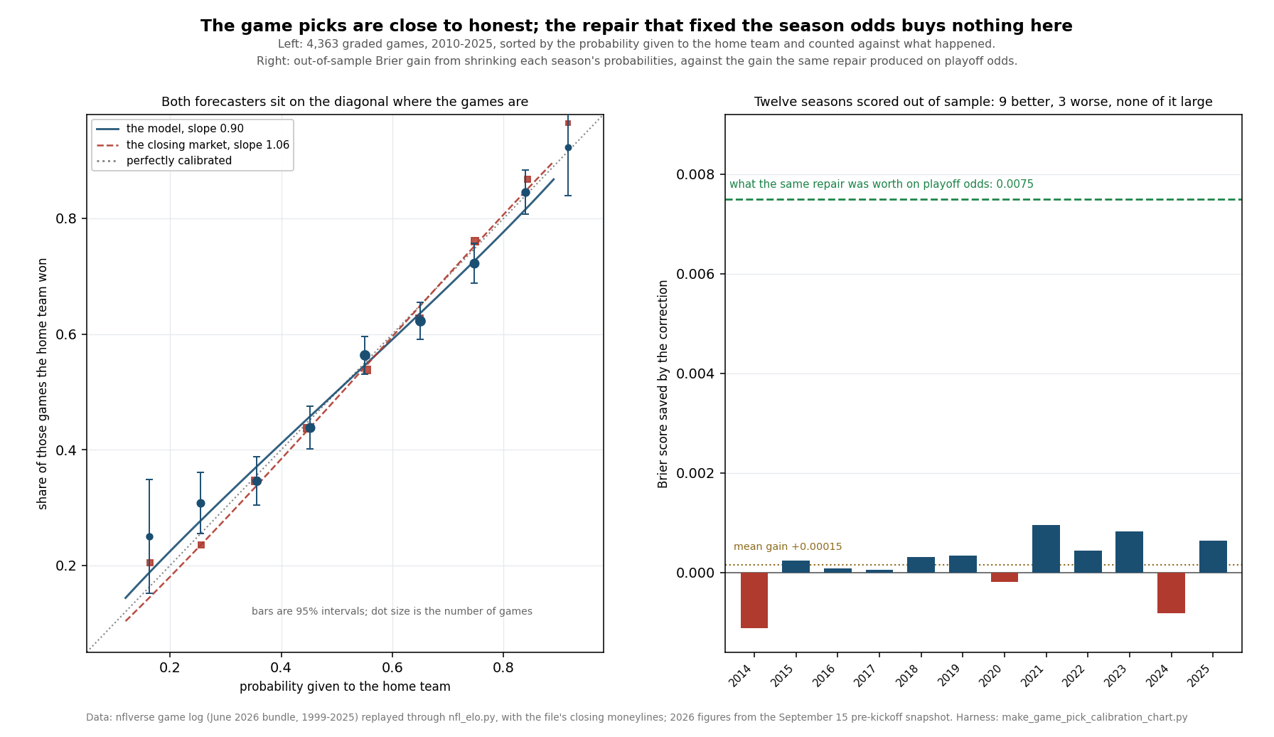
They are not. Run the identical test on the 4,363 games the engine has graded since 2010 and the game probabilities come out mildly overconfident and nearly honest: a calibration slope of 0.897 against the simulation's 0.694, with a season-clustered bootstrap standard error of 0.030. The same shrinkage, fitted only on earlier seasons and scored on 3,295 later games, moves the Brier score from .22039 to .22024. That is a gain of fifteen hundred-thousandths, about a fiftieth of what the repair was worth on playoff odds, and it is 0.9 standard errors from zero.
My position is that the slope is real, the repair is not worth shipping, and the difference between the two levels is the interesting part. The ratings are wrong by roughly the amount v68 estimated; one game is simply not a long enough lever for that error to show. A season is.
What the Replay Grades
The harness imports nfl_elo.py rather than copying it, walks the game log from 1999 in date order, prices each game before feeding it, and starts grading in 2010. It reproduces the published backtest exactly: 4,363 games graded, 4,350 decided and thirteen tied, an accuracy of .6469 and a Brier score of .2205, which is what the model page printed when the ledger opened.
Sort those games into ten bands by the probability the model gave the home team, count what happened in each, and put the market's closing price through the same mill. The market's number is the vig-free implied probability from the file's two-way moneylines, available on 4,362 of the 4,363 games.
| Probability given to the home team | Games | Stated | Home team won | 95% interval |
|---|---|---|---|---|
| 0.0 to 0.1 | 3 | 9.4% | 33.3% | ±53.3 |
| 0.1 to 0.2 | 74 | 16.2% | 25.0% | ±9.9 |
| 0.2 to 0.3 | 289 | 25.5% | 30.8% | ±5.3 |
| 0.3 to 0.4 | 504 | 35.6% | 34.6% | ±4.2 |
| 0.4 to 0.5 | 695 | 45.2% | 43.8% | ±3.7 |
| 0.5 to 0.6 | 885 | 55.1% | 56.3% | ±3.3 |
| 0.6 to 0.7 | 878 | 65.0% | 62.2% | ±3.2 |
| 0.7 to 0.8 | 652 | 74.8% | 72.2% | ±3.4 |
| 0.8 to 0.9 | 344 | 84.0% | 84.6% | ±3.8 |
| 0.9 to 1.0 | 39 | 91.6% | 92.3% | ±8.4 |
The shape is the flattening, and it is faint. The two busiest confident bands both come in under their claim, 65.0% producing 62.2% and 74.8% producing 72.2%, and the populated bands under 30% both run over: the 10-to-20 band is 8.8 points above what it promised on 74 games, the largest single gap in the table. But not one of the ten gaps clears its own 95% interval. A reader looking only at this table would have to conclude the model is calibrated, and would be making the mistake the slope catches: the misses are small, but they lean the same way on either side of the middle, and 4,363 games can see a lean that no single band can.
Fitting the whole thing at once, by logistic regression of the outcome on the log-odds of the forecast, gives a slope of 0.897 with an intercept of 0.004. A season-clustered bootstrap puts it 3.4 standard errors below one, with a 95% interval of 0.841 to 0.956 that never reaches it. The market's slope, on the same games, is 1.061, and its interval contains one. The market is calibrated; the model is a little flat; and a little is the whole finding.
The Exhibit
One Knob, Fitted Forward
The repair is the one from yesterday, in its simplest form: multiply the log-odds of each probability by lambda and turn it back into a probability. Lambda below one flattens the forecast toward a coin. Fitted on all sixteen graded seasons at once, lambda is 0.90, and leaving each season out in turn moves it only between 0.88 and 0.915. There is no knife edge here.
Fitting it on the seasons it is then scored on proves nothing, so each test season from 2014 gets a lambda chosen only from the seasons before it:
| Season | Lambda, fitted on earlier seasons | Games | Brier, as it ships | Brier, corrected | Saved |
|---|---|---|---|---|---|
| 2014 | 0.885 | 267 | 0.2049 | 0.2060 | -0.00112 |
| 2015 | 0.935 | 267 | 0.2241 | 0.2239 | +0.00024 |
| 2016 | 0.925 | 267 | 0.2178 | 0.2178 | +0.00009 |
| 2017 | 0.930 | 267 | 0.2172 | 0.2172 | +0.00006 |
| 2018 | 0.930 | 267 | 0.2221 | 0.2218 | +0.00031 |
| 2019 | 0.925 | 267 | 0.2222 | 0.2219 | +0.00035 |
| 2020 | 0.920 | 269 | 0.2145 | 0.2147 | -0.00019 |
| 2021 | 0.925 | 285 | 0.2308 | 0.2298 | +0.00095 |
| 2022 | 0.905 | 284 | 0.2234 | 0.2229 | +0.00044 |
| 2023 | 0.900 | 285 | 0.2327 | 0.2319 | +0.00083 |
| 2024 | 0.890 | 285 | 0.2098 | 0.2106 | -0.00082 |
| 2025 | 0.905 | 285 | 0.2240 | 0.2233 | +0.00064 |
Twelve test seasons, 3,295 games, better in 9 of 12. Pooled, the Brier score goes from .22039 to .22024 and the log loss from .63321 to .63263. The mean season-level gain is +0.00015 with a standard error of 0.00017, so the sign of the effect is not established at all, and the two seasons it hurt most, 2014 and 2024, cost more than any season it helped gained.
What the correction does do, reliably, is what it was built to do: the out-of-sample slope goes from 0.9005 to 0.9834. The forecast becomes better calibrated and no more accurate. That is worth stating plainly, because it is the trap in this kind of work. Calibration is a property you can fix by flattening; it is not the same thing as knowing more, and on a forecast that was already close to calibrated, fixing it buys nothing you would notice in a season.
Where the Brier Score Actually Goes
Allan Murphy's decomposition splits a Brier score into three parts: how far each band's claim sits from its outcome (reliability, lower better), how far the bands spread away from the base rate (resolution, higher better), and the variance of the outcome itself, which no forecaster can touch. On these 4,363 games:
reliability  .00067      miscalibration: 0.30% of the Brier score
resolution   .02586      what the ratings know that the base rate does not
uncertainty  .24674      home teams won .5543 of these games; this is .5543 x .4457
Brier = uncertainty - resolution + reliability = .2205
Three tenths of one per cent. Everything the site could gain by perfecting its calibration is that .00067, and the walk-forward test above recovers a fifth of it. The gap between this model and a good one is the resolution column: a forecaster that knew about quarterbacks, injuries and the previous week's news would separate the games further, not describe them more modestly. The market does exactly that, and it is why its Brier score beats this one by about a hundredth of a point a game while its calibration slope is no better behaved.
The Other Repair, and Why 120 Is the Wrong Number Here
Yesterday's preferred fix was not shrinkage but rating uncertainty: assume every rating is wrong by a normal draw of about 120 Elo points and price accordingly. That version can be run on single games too, by integrating each game's probability over the noise in the two ratings rather than simulating a season:
| Rating uncertainty (Elo points) | Brier score | Calibration slope |
|---|---|---|
| 0 (as it ships) | .22045 | 0.897 |
| 40 | .22036 | 0.918 |
| 80 | .22023 | 0.978 |
| 120 | .22031 | 1.069 |
| 160 | .22074 | 1.183 |
| 200 | .22149 | 1.313 |
The games ask for about 80 points, not 120, and even at the minimum the whole repair is worth .00022 of Brier score. Push it to the 120 the season simulation adopted and the game-level slope overshoots to 1.069: the probabilities become underconfident. So the two levels disagree about how wrong the ratings are, and the direction of the disagreement is the explanation for this whole page.
A season simulation takes one rating error and spends it 272 times. If a team's rating is fifty points too high, every one of its seventeen games is priced too high in the same direction, and the errors accumulate into a win total and then into a playoff probability that is far too extreme. A single game spends the same error once, through a logistic curve that is nearly flat where most games live: fifty Elo points is about seven points of win probability at even money, and it is a coin flip whether the error helps or hurts on any given Sunday. That is why the same underlying defect reads as a slope of 0.694 at the season level and 0.897 at the game level, and why fixing it is worth .0075 there and nothing here.
Worked Through: Seattle, and a Week That Is Already Graded
The ledger's opening game of 2026 gave Seattle .6785 at home against New England. At the fitted lambda:
logit(.6785)     = ln(.6785 / .3215)      = 0.7469
shrunk log-odds  = 0.90 x 0.7469          = 0.6722
shrunk           = 1 / (1 + e^-0.6722)    = .6620      a move of 1.65 points
That is the largest kind of move the correction makes anywhere on a sixteen-game board, and it is smaller than the rounding most people apply in their heads. Run it across the whole of 2026's graded week — the sixteen games final as of the September 15 snapshot this page reads — and the Brier score goes from .2251 to .2256. The correction made that week very slightly worse, which is exactly the coin flip the standard error above predicts.
One row of that week is worth following, because it is the one the correction should have helped. The ledger had Kansas City at .4195 at home to Denver and the Chiefs won by 21, the week's most expensive miss. Shrinking pulls that number to .4274, toward the result, and saves .0066 of Brier score on the game. Then the fifteen games it was right about each give a little of it back. A flattening cannot know which games it is rescuing, and over a season those two effects cancel to within a rounding error. That is the argument against adopting it, stated as arithmetic rather than as taste.
What This Page Does Not Show
A null is not a zero. The slope of 0.897 is genuinely below one, by three and a half standard errors, and a forecast with that slope is overconfident. What the walk-forward test rules out is that correcting it pays. Those are different claims and this page makes both.
Many cuts. Ten reliability bands, six values of rating uncertainty, a grid of 201 lambdas and twelve test seasons. The band-by-band reading is descriptive and I have said where it is too thin to lean on — three games under 10% and 39 above 90%. The claims that carry weight are the pooled slope, its bootstrap, and the out-of-sample Brier and log loss.
The lambda is fitted on the same engine. K, the home edge and the regression fraction are the published constants across the whole window. If a different K would have produced better-calibrated probabilities on its own, this test cannot see it, because it only rescales what the shipped engine produced.
The market benchmark is the file's closing prices. They carry the book's hold, which I strip proportionally; other de-vig methods move the implied probabilities by a fraction of a point and would move the market's slope a little. I have no independent record of when each price was captured.
Postseason games are pooled with regular-season ones, 188 of the 4,363, and they are played by a selected set of teams. Ties count as half an outcome in the Brier score and are dropped from accuracy.
Sixteen seasons of one league. The bootstrap resamples seasons because games inside a season share ratings and opponents. Sixteen clusters is not many, and the interval on the slope should be read as approximate.
Nothing here is about 2026's unplayed games. The only 2026 figures on this page are the sixteen week-1 results that were already final and graded when the September 15 snapshot was saved.
Method and Sources
Two files and one module. The June 2026 nflverse bundle (/data/games.csv, served at /data/games.csv), whose 7,276 rows through 2025 carry the scores and the closing moneylines, and whose 272 2026 rows are schedule only — no score, no quarterback — so nothing played in 2026 can reach these figures. The 2026 week-1 rows come from the dated pre-kickoff snapshot explainer_src/_2026_week1_snapshot_2026-09-15.json, because the build republishes the June bundle over the served copy. And explainer_src/nfl_elo.py, imported rather than copied. The harness is explainer_src/make_game_pick_calibration_chart.py. The test is these lines:
ols_logit(outcome ~ a + b * logit(p))          # b = 0.897, bootstrap SE 0.030 by season
for season in 2014..2025:                      # never fitted on itself
    lam = argmin over the grid of Brier on seasons < season
    p2  = sigmoid(lam * logit(p))
# 3,295 games: Brier .22039 -> .22024, log loss .63321 -> .63263, slope 0.9005 -> 0.9834
# the same repair on playoff odds (v68): Brier .2064 -> .1989, slope 0.694 -> 1.015
The script asserts the engine constants, the June bundle's row counts and the absence of any 2026 score or quarterback, the replay against the stored backtest game for game, the accuracy and Brier the model page published, all ten reliability bands cell by cell with their intervals, the fact that no band's gap clears its own interval, both calibration slopes and their season-clustered bootstraps, the Murphy decomposition and its sum, the full lambda grid with its leave-one-season-out range, all twelve walk-forward rows, the pooled out-of-sample scores and slopes with the season-level standard error, the rating-uncertainty sweep and its interior minimum, the snapshot's frozen scoreboard and the fact that every row it uses is a week-1 row, the worked example to four places, and this page's own figures: 80 assertions, all green as of September 17, 2026.
Sources: the nflverse public game log (games.csv), including its closing moneylines. The Brier score is Glenn Brier's, from Verification of Forecasts Expressed in Terms of Probability (1950); the three-part decomposition is Allan Murphy's, Journal of Applied Meteorology (1973); the one-parameter squash of an overconfident probability is John Platt's (1999). The rating method is Arpad Elo's.
Further reading
- Shrinking the Playoff Odds — the repair this page declines to adopt, and the level at which it pays
- Playoff Odds After Week 1 — where the 0.694 slope was measured
- The Model Cannot See a Quarterback Change — today's other page: a bias this correction would not touch
- The Model Gets Louder, Not Smarter — the same games cut by week instead of by probability
- The Model Has No Good Years, Only Lucky Ones — the season-level version of the honesty question
- Our Prediction Model, Fully Stated — the engine, its four constants, and the backtest reproduced here
- The Offseason Haircut — the engine's own admission that its ratings are wrong
- What a 60% Pick Is Worth — the market benchmark, and the gap this page attributes to resolution
- Ten of Sixteen: Kansas City 31, Denver 10, Graded — the miss the correction would have softened
- The Prediction Ledger — the published probabilities, uncorrected
- Power Rankings — the ratings every one of them is arithmetic on
Go deeper
Want the code behind these metrics? Work through the 45-chapter NFL analytics tutorial.
Browse tutorials Free tools