Four Numbers Nobody Ever Checked
The page that states this model in full lists exactly four moving parts: a K of 20, a home-field edge of 48 Elo points, a margin-of-victory multiplier, and one-third regression toward 1505 between seasons. It states them as facts. It does not say where any of them came from, and the honest answer is that three of the four came from the literature and a shrug — they are the values an Elo implementation ships with, and they were never fitted to this file.
One of the four has since been graded: the offseason-haircut page swept the regression fraction from zero to one and found the shipped third inside the defensible band, with one half marginally better on Brier score. This page does the other three, on the same 4,363 games the model reports, and then asks the question that decides whether any of it matters: does tuning them walk-forward buy anything?
My position, and the file's: the constants are fine, and the reason they are fine is not that somebody chose well. K = 20 is, to six decimal places, the best K in sixteen seasons of hindsight — 19.75 scores 0.220449 against 20's 0.220451. The home-field constant is the one that is genuinely stale, and it is stale in a way that says something about football rather than about the engine. And the part of the model that looks like decoration, the margin multiplier, is worth more than everything else on this page put together.
The Exhibit
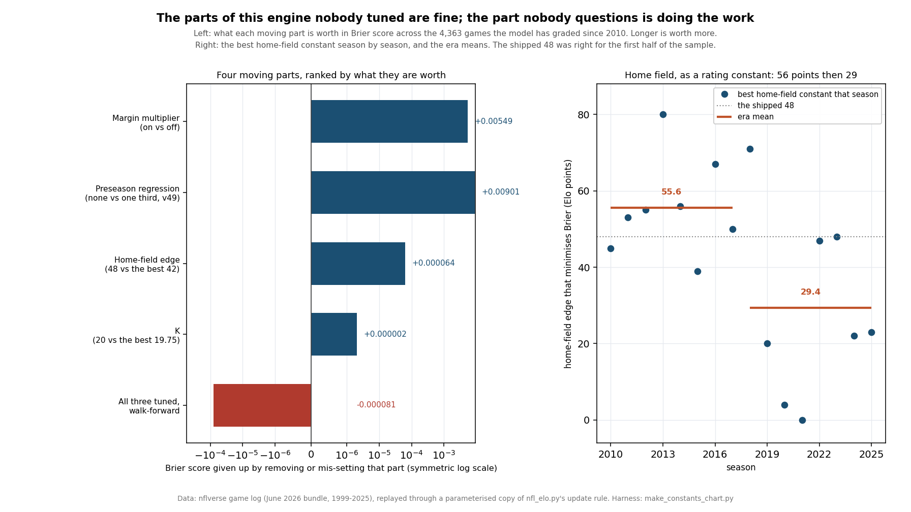
K Is Already Right, Which Is Luck
K is how fast the ratings move: after each game both teams shift by K times the gap between the result and the stated probability, scaled by the margin multiplier. Too small and the ratings never learn; too large and they chase noise. Swept from 10 to 40 in quarter-point steps, holding the other three constants at their shipped values, the Brier score bottoms out at 19.75 and the shipped 20 gives up two millionths of a point.
The curve around it is almost flat — 17 scores .22057 and 23 scores .22062, so the whole interesting range is six thousandths wide — which is the real content. A rating system fed this much data is not sensitive to K anywhere near the precision people argue about it. Anything between about 15 and 25 produces the same forecaster.
One honest complication: straight-up accuracy prefers a slower K of 17.25, at .64897 against the shipped .64690. Two tenths of a point of hit rate is not nothing, and it points the other way from the Brier score, which rewards the sharper probabilities a faster K produces. When two scoring rules disagree I take the one that grades the probability rather than the pick, because the probability is what this site publishes — but the disagreement is real and I would rather print it.
Home Field Is the One That Has Gone Stale
The engine adds 48 Elo points to the home side, waived at neutral sites. Across the full sixteen seasons the file wants 42. That is worth 0.000064 of Brier score, which is to say nothing at all — but the pooled number hides the finding:
| Window | Best home-field constant (Elo) | Home win rate | Brier at the shipped 48 |
|---|---|---|---|
| 2010–2017 | 56 | 0.5739 | 0.21833 |
| 2018–2025 | 29 | 0.5442 | 0.22248 |
| All sixteen seasons | 42 | 0.5588 | 0.22045 |
The first half of the sample wants 56 points and the second wants 29. Fitted season by season the best value averages 55.6 in the first era and 29.4 in the second, a gap of 26.2 points at t = 2.72, and the scatter is wide enough to keep honest: 80 points in 2013, zero in 2021. This is the decline the home-field page measured in raw win percentage, arriving as a rating constant — home teams won .5739 of non-neutral games in the first window and .5442 in the second.
So the shipped 48 is not a bad average. It is a good average of two different things, and it is currently about nineteen points too generous to the home side. That is the one constant I would change if the evidence below said changing constants helped. It does not.
The Part Nobody Questions Is the Part Doing the Work
The margin multiplier scales each update by the natural log of the margin plus one, damped when the winner was already a heavy favourite. It is the least discussed of the four and by far the most valuable:
| Margin treatment | Brier | Accuracy | Cost against the shipped rule |
|---|---|---|---|
| As it ships: ln(margin + 1), damped for favourites | 0.22045 | 0.64690 | +0.00000 |
| ln(margin + 1), no damping | 0.22049 | 0.64598 | +0.00004 |
| Damping only, margin ignored | 0.22615 | 0.62874 | +0.00570 |
| No multiplier at all | 0.22594 | 0.62874 | +0.00549 |
Switching the multiplier off costs .00549 of Brier score and 1.82 points of accuracy. To see how big that is, put it next to the rest of this page: the best home-field constant is worth .000064 and the best K .000002. The margin term is eighty-five times the first and two thousand times the second.
It also decomposes, and the split is not the one the model page implies. The margin term does all of it. Keeping ln(margin + 1) and throwing the favourite damping away costs four hundred-thousandths of Brier score — indistinguishable from the shipped rule. Keeping the damping and ignoring the margin is worse than having no multiplier at all, because all it does is slow every update down. The damping earns its place on accuracy, where it is worth 0.09 of a point, and essentially nowhere else.
One objection deserves answering. Turning the multiplier off makes every update smaller, so perhaps the comparison is unfair and K should be re-fitted to compensate. It should, and it is: with the multiplier off, the best K rises to 43, and even then the shipped rule is .00247 of Brier score better. Knowing that a team won by 24 rather than by 3 is worth real money, and it is the only place in this engine where that is true.
Tuning It Walk-Forward Buys Nothing
Everything above is hindsight. The test that matters is whether a tuner sitting in, say, 2018 with only earlier seasons in hand would have chosen constants that helped in 2018. So: build the whole grid — K from 4 to 40, home field from 0 to 80, regression from 0 to 1, 16,317 settings — and for each test season from 2014, pick the cell with the best Brier score on the seasons before it and score it on that season alone. Twelve test seasons, 3,284 decided games.
| Tuned walk-forward | Brier gained a season | Season SE | t | Better in |
|---|---|---|---|---|
| K only | -0.000065 | 0.000061 | -1.06 | 4 of 12 |
| Home-field edge only | -0.000023 | 0.000122 | -0.19 | 5 of 12 |
| All three jointly | -0.000081 | 0.000546 | -0.15 | 5 of 12 |
Every row is a null, and every row has the wrong sign. Tuning all three jointly loses 0.000081 of Brier score a season against a standard error of 0.000546, and beats the shipped setting in five of twelve seasons — which is what a coin does. The margin multiplier is worth more than sixty times the entire exercise.
The in-sample picture is the trap this test exists to avoid. Of the 16,317 grid cells, 513 beat the shipped setting on the full sixteen seasons — 3.1% of them — and the best of those, K 22 with a 40-point home edge and half-way regression, gains .00073. Leaving each season out in turn picks that same cell ten times of sixteen, so it is not unstable in the usual sense. It is simply the best of sixteen thousand tries on 4,363 games, and it does not survive contact with a season it has not seen. A grid this size hands out gains of that order for free.
Worked Through: What Nineteen Points of Home Field Is
The era finding is the only one on this page with a number large enough to feel, so here it is priced on the simplest possible game — two teams with identical ratings, one of them at home:
p(home) = 1 / (1 + 10 ** (-edge / 400))

edge = 56 (what 2010-2017 wanted)                  = .5799
edge = 48 (what the engine uses)                   = .5686
edge = 42 (what all sixteen seasons want)          = .5602
edge = 29 (what 2018-2025 wanted)                  = .5416
Between the two eras that is 3.83 points of win probability on a coin-flip game, and the engine sits nearer the older half. On the 2026 board the same arithmetic is why three of the sixteen openers were priced with the host favoured despite the visitor carrying the better rating: a flat 48 does proportionally more work once the preseason haircut has squeezed the ratings together.
And for the whole grid at once, the frozen August board rebuilt with the best in-sample cell — K 22, home field 40, half regression — reads Seattle 1642.0 against the published 1674.6, with the spread between best and worst team falling from 324.8 rating points to 252.7. Only one team moves more than two places: Buffalo, four places lower. Sixteen thousand settings, one re-rank worth arguing about, and no out-of-sample gain.
What This Page Does Not Show
Sixteen thousand comparisons. That is the entire methodological point and it cuts both ways: the 3.1% of cells that beat the shipped setting are what a grid this size produces by chance, and so, potentially, is the 56-against-29 era split. That one I would defend, because it has an independent corroborating measurement in the raw home win rate and a t of 2.72, but it is one cut of many.
A null is not proof the constants are optimal. What the walk-forward test rules out is that a tuner could have done better in advance. It does not rule out that a different form of model — a time-varying home edge, a K that depends on the week, an asymmetric regression — would beat this one. Those are different models, not different constants, and this page does not test them.
The regression axis is not mine. It was swept on the haircut page, whose table this harness reproduces row for row, and it is included in the joint grid only so the three can be tuned together. Reading the joint result as new evidence about the regression fraction would be double-counting.
Twelve test seasons is twelve observations, and the standard errors are computed across them because games inside a season share ratings and opponents.
Brier and accuracy disagree about K, and the page picks Brier. A reader who cares only about straight-up picks should read the K section as saying 17 rather than 20, and should note that the difference is two tenths of a point on 4,350 games.
Everything here is history. The grading window is 2010 to 2025, with 1999 to 2009 as burn-in, and the only 2026 figures are the frozen August ratings locked on 2026-08-12 from 2025 results. No game played this season touches a number on this page.
Method and Sources
One file and one module. The June 2026 nflverse bundle (/data/games.csv, served at /data/games.csv): 7,276 games played from 1999 to 2025, its 272 2026 rows schedule-only. And explainer_src/nfl_elo.py, whose constants and update rule the harness reproduces in a parameterised copy — a copy rather than an import, because the point is to vary the constants, and the copy is checked against the module by reproducing the published backtest exactly at the shipped values: 4,363 games graded, Brier .2205, accuracy .6469. The harness is explainer_src/make_constants_chart.py. The grid is these lines:
for K in 4..40, HFA in 0..80, REG in 0..1:          # 16,317 settings
    agg[K, HFA, REG] = replay(K, HFA, REG)          # one walk-forward pass each

for season in 2014..2025:                           # never fitted on itself
    cell = argmin over the grid of Brier on seasons < season
    score(cell, season)
# 3,284 decided games: -0.000081 of Brier a season, season SE 0.000546
The script asserts the engine constants, the bundle's row counts and the absence of any 2026 score, the replay against the published backtest, the haircut page's regression sweep row for row, the fine K sweep with its optimum and the accuracy disagreement, the fine home-field sweep with both era optima and their per-season standard errors, the raw home win rates behind them, all four margin treatments and the re-fitted K with the multiplier off, the size of the full grid, the best cell and the count that beats the shipped setting, the leave-one-season-out stability, all three walk-forward arms with their standard errors, the frozen August board reproduced and rebuilt, the worked example to four places, and this page's own figures: 55 assertions, all green as of September 19, 2026.
Sources: the nflverse public game log (games.csv). The rating method is Arpad Elo's, from The Rating of Chessplayers, Past and Present (1978); the margin-of-victory multiplier follows the form popularised by Nate Silver's NFL Elo write-ups; the Brier score is Glenn Brier's (1950).
Further reading
- Our Prediction Model, Fully Stated — the four constants, stated but never graded until now
- The Offseason Haircut — the fourth constant, already swept, and the source of the regression row here
- Home-Field Advantage, Measured — the decline this page finds again as a rating constant
- What One Game Moves — the update rule K and the margin multiplier act on
- Three Fixes, One Knob — today's other page: corrections applied to the output rather than the constants
- Shrinking the Playoff Odds — where a single parameter did pay, at the season level
- Where the Overconfidence Is Not — the same walk-forward discipline applied to the probabilities
- The Model Gets Louder, Not Smarter — the same replay cut by week of season
- The Week 10 Problem That Isn't — another result that survives only until it is tested properly
- The Prediction Ledger — every probability these constants produce
- Power Rankings — the ratings K and the home edge build
Go deeper
Want the code behind these metrics? Work through the 45-chapter NFL analytics tutorial.
Browse tutorials Free tools