The Multiplier Earns Its Place. The Curve Does Not.
Yesterday this site graded its own engine's constants and found the surprise sitting where nobody had looked. K is already optimal and the home-field edge is worth millionths, but the margin-of-victory multiplier — the term that looks like decoration — is the one part of the update rule that is genuinely load-bearing. Strip it out and re-fit K to compensate, and the model is still 0.002470 of Brier score worse over the 4,363 games it has graded since 2010.
That page stopped there, and it left the obvious question unasked. The multiplier is a specific function: the natural log of the margin plus one. Why that one? An Elo implementation could scale its updates by the margin itself, by the square root of the margin, by the margin capped at three touchdowns, or by any of a hundred other increasing curves. If the margin term is worth real money, the particular shape ought to be worth something too.
It is worth almost nothing, and that is my position on this page. Once K is allowed to rescale the update — which it must be, because a steeper curve makes every update bigger and that is a question about size, not shape — the whole range of sensible curves collapses into one forecaster. Across the power curves from the fourth root of the margin to the margin itself, the entire spread in Brier score is 0.000507, against the 0.002816 that separates the best of them from ignoring margin altogether. The engine's log is not a good choice. It is one of a great many choices that are all the same choice.
Where the file does argue with the log is at the bottom of the scale, and the argument is one this site has published before in a different form: fitted freely, the data wants a three-point win and a seven-point win treated as the same event.
The Exhibit
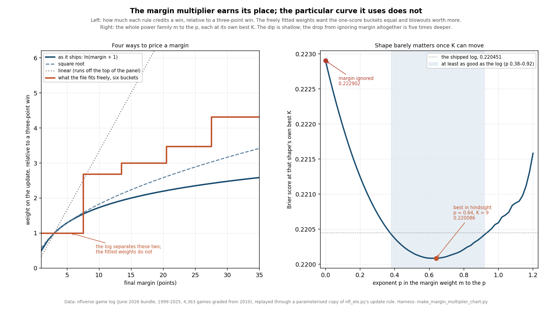
Shape Barely Matters Once K Can Move
The comparison has to be done carefully or it is meaningless. Swapping the log for the raw margin multiplies every update by roughly eight, so at a fixed K = 20 the linear rule would look catastrophic — and the catastrophe would be that the ratings are lurching, not that the shape is wrong. So every rule below is given its own best K, swept from 2 to 81 in half-point steps, and judged only after that.
| How the margin enters the update | Its own best K | Brier | Accuracy | Against the shipped rule |
|---|---|---|---|---|
| Margin ignored entirely | 45.0 | 0.222902 | 0.63816 | +0.002451 |
| Linear, the margin itself | 3.0 | 0.220593 | 0.64368 | +0.000142 |
| Square root of the margin | 14.0 | 0.220169 | 0.64759 | -0.000282 |
| As it ships: log of the margin plus one | 19.5 | 0.220449 | 0.64667 | -0.000002 |
| The best exponent in the family, m to the 0.64 | 9.0 | 0.220086 | 0.64713 | -0.000365 |
Read the last column. The gap between the best shape anyone can find in hindsight and the worst one on the table — raw linear margin, the rule the logarithm exists to protect against — is five ten-thousandths of a point. The gap between any of them and the row at the top, where margin carries no information at all, is five times larger. Whatever the multiplier is doing for this model, it is doing it as soon as the update knows that twenty-eight points is more than three. The precise exchange rate between them is a rounding error.
The full sweep says the same thing more completely. Taking the weight as the margin raised to the power p and letting K re-fit at every step, the Brier score bottoms out at p = 0.64 with K = 9, at 0.220086 against the shipped 0.220451. That is a hindsight gain of 0.000365. Everything from p = 0.50 to p = 0.78 is within a ten-thousandth of that floor, and 28 of the 61 exponents tested — from 0.38 to 0.92 — are at least as good as the log. The log itself behaves like an exponent of about 0.4 over the range of margins football actually produces, which is why it lands where it does.
One disagreement worth printing, because it points the other way from the headline. Straight-up accuracy prefers a squarer curve than Brier does: p = 0.48 hits .64920 against the shipped .64690, about a quarter of a point of hit rate. As on yesterday's page, when the two scoring rules disagree I take the one that grades the probability rather than the pick, because the probability is what this site publishes. But the disagreement is real.
Where the File Does Disagree With the Log
A power curve is still a smooth, committed shape. The sharper test is to throw the functional form away entirely: cut the margins into six buckets, give each one a free weight, and let the file choose all six by coordinate descent with K re-fitted after every pass. The result is the most interesting thing on this page.
| Final margin | Games | What the log gives it | What the file fits |
|---|---|---|---|
| 1–3 | 1,698 | 1.00 | 1.00 |
| 4–7 | 1,708 | 1.70 | 1.00 |
| 8–13 | 1,281 | 2.22 | 2.68 |
| 14–20 | 1,289 | 2.63 | 3.00 |
| 21–27 | 741 | 2.93 | 3.47 |
| 28 or more | 544 | 3.21 | 4.32 |
Both columns are scaled to the one-score bucket, so only the ratios matter. Two things are going on, and they pull in opposite directions.
The log discriminates where the file does not. It gives a four-to-seven-point win 1.70 times the weight of a one-to-three-point win. The free fit gives the two buckets exactly the same number. That is not a subtle result to anyone who has read the one-score-games page, which puts half of all NFL games inside a single possession and argues that the margin inside that band is mostly noise about which drive stalled — or the close-game page, which shows one-score records failing to persist at all. The update rule arrives at the same conclusion from a completely different direction: as evidence about who is better, a field goal and a touchdown are the same game.
And the log under-credits routs. The fit wants a 28-point win worth 4.32 times a one-score win, where the log offers 3.21. The logarithm flattens hard by construction — that is the whole reason it is there, and the update-rule page made the point that the difference between winning by 24 and winning by 31 is mostly garbage time. The file's answer is that the flattening is slightly overdone at the top and badly overdone at the bottom.
In sample, six free weights plus a re-fitted K score 0.219806, a gain of 0.000644 over the shipped rule. Forcing the second bucket back to the log's ratio while leaving the other five alone costs 0.000218 of that, so a little over a third of the gain is the one-score finding by itself.
I would hold the bottom half of this more firmly than the top. The second bucket's profile is shallow — anything from 0.60 to 1.20 costs less than six hundred-thousandths — so the exact equality is not pinned down. What is pinned down is the direction: nowhere in the plausible range does the file want the 1.70 the log is currently applying.
Tuning the Shape Forward Buys Nothing
Everything above is hindsight, and the grid is large enough to manufacture hindsight. Of the 4,697 combinations of exponent and K that were swept, 206 beat the shipped rule on the full sixteen seasons — 4.4% of them — which is roughly what a grid that size hands out for free.
So the test that decides it: for each season from 2014, choose the setting that scored best on the seasons before it alone, and grade that choice on the season it has never seen. Twelve test seasons, 3,295 graded games, and the same discipline for both of the repairs above.
| Fitted only on earlier seasons | Brier gained a season | Season SE | t | Better in |
|---|---|---|---|---|
| The exponent and K, chosen from the 4,697 | −0.000424 | 0.000844 | −0.50 | 6 of 12 |
| Six free bucket weights and K | −0.000521 | 0.000651 | −0.80 | 5 of 12 |
Both are nulls, both have the wrong sign, and the one with the larger in-sample gain has the worse out-of-sample record. Six of twelve and five of twelve is what a coin does. The exponent the tuner selects wanders from 0.66 to 1.12 across those twelve seasons without ever settling, which is the honest signature of a parameter the data cannot locate: the objective is so flat near its floor that each new season's noise moves the argmin a long way without moving the score.
That is the second time in two days this has happened here, and the pattern is worth naming. The page on combining corrections found three separately-fitted repairs collapsing into one; yesterday's constants page found joint tuning gaining −0.000081. A model this simple, fed this much data, appears to have very few knobs that repay turning, and the margin term is valuable precisely because it is not a knob — it is the difference between using a piece of information and discarding it.
A Test That Never Touches the Brier Score
Every number so far is the engine grading itself, which is a closed loop worth escaping. Here is an independent check on whether the shipped update is the right size, using no Brier score at all.
If the multiplier under-reacts to blowouts, then a team that has just won by thirty is still under-rated going into its next game, and it should beat its next stated probability on average. If it over-reacts, the opposite. So take every pair of consecutive games by the same team in the graded window — 8,188 of them — and regress the residual from the second game, outcome minus the probability the engine published, on the margin of the first.
The slope is +0.000399 of probability per point of margin, with a season-clustered standard error of 0.000347. That is 1.15 standard errors from zero. A twenty-point win leaves its winner about eight tenths of a point of win probability under-rated for the next week, and the interval comfortably contains nothing at all.
| How the last game went | Team-games | Next game, outcome minus probability | SE |
|---|---|---|---|
| Lost by 21 or more | 686 | -0.0012 | 0.0180 |
| Lost by 14 to 20 | 700 | -0.0155 | 0.0173 |
| Lost by 8 to 13 | 676 | -0.0182 | 0.0178 |
| Lost by 1 to 7 | 1,911 | +0.0010 | 0.0109 |
| Won by 1 to 7 | 2,013 | +0.0037 | 0.0105 |
| Won by 8 to 13 | 711 | +0.0203 | 0.0175 |
| Won by 14 to 20 | 753 | -0.0157 | 0.0173 |
| Won by 21 or more | 738 | +0.0214 | 0.0172 |
Not one of the eight bands misses by two of its own standard errors, and the two that look most suggestive point opposite ways: teams coming off a 21-point win beat their next number by 2.1 points of probability, teams coming off a 14-to-20-point win miss theirs by 1.6. Eight bands will produce a pair like that regularly with nothing underneath. The pooled slope is the number to use, and the pooled slope says the shipped compression is about right, with whatever bias remains pointing very slightly toward under-reaction — the same direction the free bucket fit pointed, at a size neither test can distinguish from zero.
Worked Through: A Field Goal and a Rout, Priced Identically Beforehand
The cleanest illustration in the file is a pair of games the engine walked into with exactly the same opinion. In week 2 of 2016 Minnesota hosted Green Bay; in week 13 of the same season Baltimore hosted Miami. Both hosts were rated a shade better than their visitors, and the replay priced both at .5465 — the two probabilities agree to five decimal places. Then one game was decided by a field goal and the other by thirty-two points.
Minnesota 17, Green Bay 14                     Baltimore 38, Miami 6
  gap  = 1578.4 + 48 - 1594.1 = 32.3             gap  = 1492.4 + 48 - 1508.0 = 32.4
  p    = .5465                                   p    = .5465
  damping = 2.2 / (0.001 * 32.3 + 2.2) = .98553  damping = .98549

as it ships, ln(margin + 1) at K = 20
  20 * ln(4)  * .98553 * (1 - .5465)  = 12.392   20 * ln(33) * .98549 * .4535 = 31.256
linear margin at its own best K = 3
  3 * 3 * .98553 * .4535 = 4.023               3 * 32 * .98549 * .4535 = 42.909
The shipped rule pays the rout 2.52 times what it pays the field goal. The linear rule, scaled so that its average update across the file is comparable, pays it 10.67 times as much — and pays the three-point win almost nothing, four rating points, because a three-point game is a small number and linear scaling takes small numbers literally. The two rules disagree violently about these two nights. Over 4,363 games they disagree by 0.000142 of Brier score.
That is the whole argument in one pair. The shapes differ enormously game by game, and the differences wash out, because the margins that separate the rules most are rare — the average winning margin in the file is 11.544 points, 17.7% of games end by 21 or more, and only 7.5% by 28 or more — while the margins where every rule agrees are the bulk of the schedule. The log's real work is done in the crowded middle, where it is indistinguishable from its rivals.
What This Page Does Not Show
Thousands of comparisons. 4,697 grid cells, 61 exponents, six free weights fitted by search, and eight residual bands. The 206 cells that beat the shipped rule in hindsight are what a search that size produces by chance, and so, potentially, is the bucket fit. The walk-forward columns are the only real protection, and they protect the parameter choice rather than the decision to go looking.
The damping factor is held fixed throughout. The shipped multiplier has a second term that shrinks updates when the winner was already a heavy favourite. Yesterday's page graded it and found it worth essentially nothing on Brier score; every rule here carries it unchanged, so none of these comparisons speaks to it. Re-fitting K makes that finding slightly stronger, incidentally: with the margin term gone, damping on and damping off score within two hundred-thousandths of each other.
A null on shape is not a licence to pick any shape. What is ruled out is that switching the log for another concave curve would measurably help this model on this data. Curves far outside the range tested — a rule that ignores everything past a touchdown, say, or one that grows faster than linearly — are not covered, and the left end of the right-hand panel shows how fast the score deteriorates once the curve stops being informative.
Brier and accuracy disagree about the exponent, as they disagreed about K. A reader who cares only about straight-up picks should read the sweep as preferring something nearer a square root, and should note that the difference is a quarter of a point on 4,350 decided games.
Twelve test seasons is twelve observations. The standard errors are computed across seasons rather than games, because games inside a season share ratings and opponents, and twelve is not many.
The residual test inherits the engine's ratings. It asks whether the shipped update was the right size given everything else the shipped model believes. A different K or a different home-field constant would move it, and it cannot separate an error in the multiplier from an offsetting error elsewhere.
Everything here is history. The grading window is 2010 to 2025, with 1999 to 2009 as burn-in. The harness reads the bundled game log and the engine module, and nothing else — no ledger, no scoreboard, no current rating. No game played this season touches a number on this page.
Method and Sources
One file and one module. The June 2026 nflverse bundle (/data/games.csv, served at /data/games.csv): 7,276 games played from 1999 to 2025, its 272 2026 rows schedule-only and scoreless. And explainer_src/nfl_elo.py, whose update rule the harness reproduces in a parameterised copy — a copy rather than an import, because the point is to vary the margin term, and the copy is checked against the module by reproducing the published backtest at the shipped settings: 4,363 games graded, Brier .2205, accuracy .6469. The harness is explainer_src/make_margin_multiplier_chart.py. The substitution is one line:
multiplier = f(|margin|) * (2.2 / (0.001 * |adjusted gap| + 2.2))
shift      = K * multiplier * (outcome - p_home)

for f in {ln(m+1), m, sqrt(m), m**p for p in 0..1.2, six free bucket weights}:
    K = argmin over 2..81 of Brier(f, K)        # every shape judged at its own scale

for season in 2014..2025:                       # never fitted on itself
    cell = argmin over the grid of Brier on seasons < season
    score(cell, season)
# 3,295 graded games: -0.000424 of Brier a season, season SE 0.000844
The script asserts the engine constants, the bundle's row counts and the absence of any 2026 score, the replay against the published backtest and the shipped rule's average move, yesterday's two figures reproduced at K = 20 and the re-fitted cost of removing the margin term, the full 61-point exponent sweep with its minimum, its flat band and the band that matches the log, all five named shapes at their own best K with their accuracies, the six fitted bucket weights against the log's ratios with the cost of forcing the second one back, the shallowness of that bucket's profile, the size of the grid and the count that beats the shipped rule, both walk-forward arms with their season standard errors and win counts and the wandering exponent, the residual regression with its clustered standard error and all eight bands, the two worked-example games down to their scores, ratings and both shifts, the margin distribution behind them, and this page's own figures: 68 assertions, all green as of September 20, 2026.
Sources: the nflverse public game log (games.csv). The rating method is Arpad Elo's, from The Rating of Chessplayers, Past and Present (1978); the margin-of-victory multiplier follows the form popularised by Nate Silver's NFL Elo write-ups; the Brier score is Glenn Brier's, from Verification of Forecasts Expressed in Terms of Probability (1950); season-clustered standard errors follow Liang and Zeger, Biometrika (1986).
Further reading
- The Constants Nobody Tuned — where the margin term was found to be the valuable one, and the damping factor this page holds fixed
- What One Game Moves — the update rule game by game, and why the log flattens blowouts on purpose
- Are Half of All NFL Games Really One-Score Games? — the half of the schedule the fitted weights refuse to distinguish
- One-Score Records Are Luck — the same conclusion reached from team records rather than from the update rule
- Key Numbers: Why 3 and 7 Matter — the margin distribution every rule on this page is averaging over
- Our Prediction Model, Fully Stated — the engine, its four constants, and the backtest this harness reproduces
- Three Fixes, One Knob — another set of repairs that collapsed under the same walk-forward discipline
- The Offseason Haircut — the fourth constant, swept on its own axis
- The Model Gets Louder, Not Smarter — the same replay cut by week of season
- The Week-2 Line Moves Just Enough — the market's version of the right-sized update
- The Prediction Ledger — every probability this update rule produces
- Power Rankings — the ratings the multiplier builds, one game at a time
Go deeper
Want the code behind these metrics? Work through the 43-chapter NFL analytics tutorial.
Browse tutorials Free tools