The Pattern Was Real. It Was Also Useless.
Sunday's six misses averaged 33.0 combined points. Its eight correct picks averaged 42.9. The lowest-scoring game on the board, Minnesota 9 at Chicago 3, was a miss; the two highest, Dallas 37–20 and Kansas City 33–30, were both hits. Yesterday's grading note declined to read anything into a fourteen-game slate, which was the right call for the things it was refusing. This is the one pattern in that slate worth following, because it comes with a mechanism: a low-scoring game has fewer possessions, fewer possessions means the better team gets fewer chances to be the better team, and a forecast built on ratings should therefore land less often.
It does. Across the 4,350 games this engine has graded since 2010, sort them into equal fifths by final combined points and the lowest fifth — games at 27 points on average — grades at 62.2% against a claimed 65.1%. The best bucket, games landing between 48 and 56, grades at 67.3%. That is a five-point spread in accuracy, and the Brier score moves with it: .2299 in the lowest bucket against .2087 in the best.
Then it falls apart, in two stages, and my position is that the second stage is the one worth learning. Sort the same 4,350 games by the pregame total line instead — the one version of "this will be a low-scoring game" you can have before kickoff — and the gradient disappears. The correlation between the final total and whether the pick landed is +.0287. Between the pregame line and whether the pick landed it is +.0085, on a standard error of .0152. The market's best estimate of how much scoring is coming tells you nothing about whether this model is about to be wrong.
The Exhibit
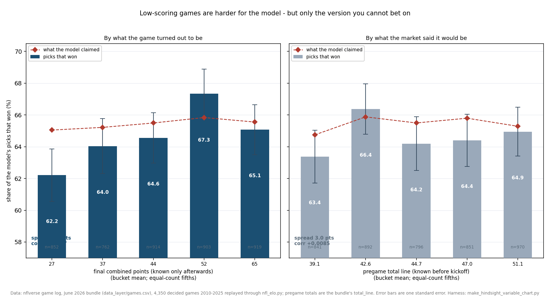
Both Sorts, Side by Side
| Sorted by final combined points | Games | Claimed | Won | Gap | Brier |
|---|---|---|---|---|---|
| Under 34 — mean 27 | 852 | 65.05% | 62.21% | −2.84 | .2299 |
| 34–40 — mean 37 | 762 | 65.22% | 64.04% | −1.18 | .2254 |
| 41–47 — mean 44 | 914 | 65.49% | 64.55% | −0.94 | .2230 |
| 48–56 — mean 52 | 903 | 65.84% | 67.33% | +1.49 | .2087 |
| 57 and up — mean 65 | 919 | 65.55% | 65.07% | −0.48 | .2192 |
| Sorted by pregame total line | Games | Claimed | Won | Gap | Brier |
|---|---|---|---|---|---|
| Under 41.5 — mean 39.1 | 841 | 64.75% | 63.38% | −1.37 | .2283 |
| 41.5–44 — mean 42.6 | 892 | 65.88% | 66.37% | +0.49 | .2156 |
| 44–46 — mean 44.7 | 796 | 65.50% | 64.20% | −1.30 | .2243 |
| 46–48.5 — mean 47.0 | 851 | 65.80% | 64.39% | −1.40 | .2212 |
| 48.5 and up — mean 51.1 | 970 | 65.29% | 64.95% | −0.34 | .2167 |
The top table has a shape. The bottom table has five numbers between 63.4 and 66.4 in no order at all, and its largest single gap belongs to the second bucket, not the lowest. Same games, same model, same bucket sizes. The only difference is whether the sorting variable was available before kickoff.
How Big Is the Real Effect? Smaller Than It Looks
Before drawing a lesson from the top table, the top table deserves a harder look, because I do not think it is as solid as its shape suggests.
Compare the lowest-scoring fifth against the other four together. The low bucket grades 62.21% over 852 games; everything else grades 65.29% over 3,498. The difference is 3.09 percentage points:
p1 = 0.6221  n1 =  852        p2 = 0.6529  n2 = 3498
diff = 0.0309
se   = sqrt( p1(1-p1)/n1 + p2(1-p2)/n2 ) = 0.0185
z    = 0.0309 / 0.0185 = 1.67
z = 1.67. That is short of the conventional threshold, and it should be read as short of it by more than the arithmetic suggests, because this hypothesis did not arrive from theory. It arrived from looking at one Sunday, noticing that the misses were the low-scoring games, and then going to find out whether that held. That is the wrong order, and it is exactly the order that turns noise into findings. A test built to confirm something you have already seen needs a higher bar than 1.67, not a lower one.
The whole-sample correlation says the same thing more bluntly. At n = 4,350 the standard error on a correlation is .0152. The final-total correlation of +.0287 is 1.9 standard errors; the pregame-line correlation of +.0085 is barely half of one. Neither is the kind of number anyone should build a model change on. The first one is at least pointing somewhere.
Why the Forecastable Version Is Flat
The obvious objection is that the pregame total is simply a bad forecast of the final total, so of course the gradient washes out. It is not a bad forecast. Across the same 4,350 games the mean line is 45.05 and the mean final total is 45.56 — the market is off by half a point on average, which is about as unbiased as an NFL number gets, a result this site has measured directly.
The market is unbiased and still useless here, and the two facts sit together comfortably once you separate the average from the scatter. A total line is a good estimate of the mean of a distribution whose spread is enormous: individual games miss their line by a 13.4-point standard deviation. A game listed at 39.0 is genuinely more likely to land under 34 than a game listed at 51.0, but it is nowhere near certain to, and the low-scoring games that actually hurt the model are scattered across every bucket of the line.
Put it the other way round, which is the version that matters for a forecaster: the thing that makes a game hard for this model is not that it was expected to be low-scoring. It is that it came out low-scoring — the defensive slog, the two turnovers inside the twenty, the rain nobody priced. Those are realisations, not conditions. You cannot bet on a realisation and you cannot condition a pregame probability on one.
That distinction is worth more than the effect it kills. A variable that predicts your errors is only worth having if you hold it before you commit. This site has already retired one repair for exactly this reason: the quarterback-change correction is worth 78 Elo points in hindsight and cannot be applied forward, because nobody knows in September who will change quarterback in November. Final scoring is the same defect wearing different clothes.
Worked Through: Sunday Under Both Sorts
The slate was genuinely low-scoring. Its fourteen games averaged 38.6 combined points against the sixteen-year mean of 45.6, which puts it in the bottom quarter of the 298 slates of thirteen or more games in the dataset. Three of the fourteen had a team score three points or fewer.
So the hindsight sort explains Sunday well. The forecastable sort does not get the chance to: at the moment the picks were locked, the model knew the ratings and the schedule, and nothing in what it knew said "this will be the fortnight's ugly slate". Take the two extremes:
Minnesota at Chicago   pick CHI at 53.4%   final  9- 3  =  12 pts   MISS
Indianapolis at KC     pick KC  at 70.1%   final 33-30  =  63 pts   HIT

after the fact: only 14 of the 4,350 games finished at 12 points or fewer
before kickoff: nothing separated these two games except the ratings themselves,
                which is the information the 53.4% and the 70.1% already contain
The Chicago pick was a 53.4% coin flip that lost, and the model said so at the time. Reclassifying it afterwards as "one of the hard ones" adds nothing, because the 53.4% had already said it was hard. That is the trap in the top table: it looks like a correction waiting to be applied, and what it actually describes is information the probability was already carrying.
What This Page Does Not Show
The hypothesis was generated by the data it is tested on, once removed. Sunday suggested it; history tested it. That is better than testing it on Sunday, and it is worse than having predicted it in advance. I have reported the test as weak rather than rounding 1.67 up into a finding.
Five buckets is a choice, and so is the variable. Equal-count fifths on combined points is one of many defensible cuts. I did not sweep bucket counts looking for a version with a bigger gap, and if I had, the first thing to say about any gap that appeared would be that I went looking for it.
This is not a claim that scoring environment is irrelevant to football. It is a narrow claim about one rating model's pick accuracy: the pregame total line does not improve it. Other models, and other questions about the same games, may well find the line informative.
No closing lines are used. The bundle's total_line is the game's listed total as nflverse records it, not a verified close, and this page makes no claim about any market's efficiency or about what anything would have returned.
Sunday's fourteen games are not part of the 4,350. The historical replay ends in 2025. The slate appears here only as the thing that raised the question.
Method and Sources
One file: the June 2026 nflverse bundle (/data/games.csv, served at /data/games.csv), replayed game by game through explainer_src/nfl_elo.py with 1999–2009 as burn-in and 2010–2025 graded — 4,350 decided games, every one of them carrying a pregame total line. The bundle's 2026 rows are schedule-only and scoreless, and the harness asserts that before it starts, so no live result reaches a historical figure. Sunday's own fourteen games are read from the pin yesterday's page captured (_honest_not_sharp_2026-09-21.json), because a site build republishes the June bundle over the served 2026 scores.
for each graded game:
    p    = engine probability on the side it picked
    hit  = 1 if that side won
    tot  = home_score + away_score      # known only afterwards
    tl   = total_line                   # known before kickoff

for key in (tot, tl):
    five equal-count buckets by key
    report claimed = mean p, actual = mean hit, and their gap
    corr(key, hit) against a standard error of 1/sqrt(n-3)
The harness is explainer_src/make_hindsight_variable_chart.py. It asserts the bundle carries no 2026 score; the replay's game count and its reproduction of the published backtest at .6469 accuracy and .2210 Brier; that every graded game has a total line, and the two mean totals; both sets of quintile cuts, that all ten buckets hold between 700 and 1,000 games and that each set partitions the sample exactly; every claimed rate, actual rate, gap and Brier in both tables; that the lowest-scoring bucket is the worst of its five on both measures; that the final-total spread exceeds five points while the total-line spread stays under three; both correlations, their shared standard error and the ratio between them; the two-proportion test down to its z; and from the pin, Sunday's split of six misses and eight hits with their mean totals, the slate mean, its rank among the 298 comparable slates in the bundle, the twelve-point Minnesota game and the three teams held to three points or fewer: 68 assertions, all green as of September 21, 2026.
Sources: the nflverse public game log (games.csv), whose total_line field supplies every pregame total. The rating method is Arpad Elo's, from The Rating of Chessplayers, Past and Present (1978); the Brier score is Glenn Brier's, from Verification of Forecasts Expressed in Terms of Probability (1950).
Further reading
- A Worse Score Is Not a Worse Model — the grading note this page follows up, and the pin it reads Sunday from
- The Model Cannot See a Quarterback Change — the other correction that works only in hindsight
- How Accurate Is the Over/Under? — the unbiased-but-scattered total line this page leans on
- Three Fixes, One Knob — three more repairs that did not survive being tested properly
- The Model Gets Louder, Not Smarter — the same replay cut by week instead of by scoring
- Are Half of All NFL Games Really One-Score Games? — the margin distribution underneath the low-scoring bucket
- NFL Scoring by Week — when in the season the low-scoring games actually fall
- The Most Common Final Scores in the NFL — why 9–3 and 20–3 look stranger than they are
- Weather and NFL Scoring — one of the realisations that turns a priced game into an ugly one
- Our Prediction Model, Fully Stated — the engine being graded here
- The Prediction Ledger — every live pick, with its locked date
Go deeper
Want the code behind these metrics? Work through the 45-chapter NFL analytics tutorial.
Browse tutorials Free tools